Building a Discounted Cash Flow (DCF) Model: A Step-by-Step Guide

A Discounted Cash Flow (DCF) model is the gold standard for valuing businesses, projects, or assets.
By forecasting future cash flows and discounting them to today’s dollars, it helps investors determine whether an opportunity is undervalued or overvalued.
In this guide, we’ll break down how to build a DCF model from scratch, including calculating free cash flow, discount rates, terminal value, and interpreting results. Let’s dive in!
Step 1: Calculate Free Cash Flow (FCF)
Free Cash Flow (FCF) represents the cash a company generates after covering operating expenses and capital expenditures. It’s the lifeblood of the DCF model.
Formula:
FCF = Operating Cash Flow (OCF) - Capital Expenditures (CapEx) - Changes in Working Capital (NWC)
Breaking it down:
- Operating Cash Flow (OCF): OCF = EBIT × (1 - Tax Rate) + Depreciation & Amortization
- CapEx: Cash spent on long-term assets (e.g., machinery, buildings)
- Changes in Working Capital (NWC): Fluctuation in a company's short-term financial position
Example:
- EBIT = $10M
- Tax Rate = 25% → After-tax EBIT = $7.5M
- Depreciation = 2M→7.5M + 2M=$9.5M
- CapEx = 3M→9.5M - 3M=$6.5M
- NWC = 1.5M→6.5M - 1.5M=$5.0M
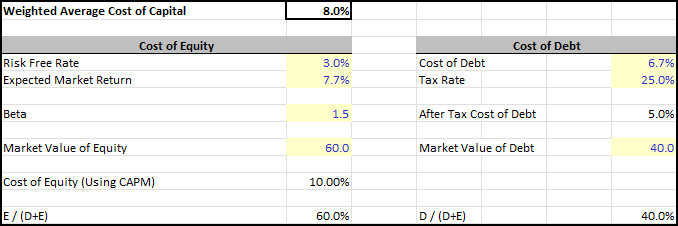
Step 2: Calculate the Discount Rate (WACC)
The Weighted Average Cost of Capital (WACC) reflects the blended cost of debt and equity. It’s used to discount future cash flows to their present value.
Formula:
WACC = (E/V × Re) + (D/V × Rd)
- E = Market value of equity
- D = Market value of debt
- V = Total value (E + D)
- Re = Cost of equity (Use CAPM)
- CAPM: (Equity Risk Premium x Beta) + Risk-Free Rate
- Equity Risk Premium = Expected Market Return - Risk-Free Rate
- Rd = Cost of Debt (After Tax)
- Interest rate on debt × (1 - Tax Rate)
Example:
- Equity = 60M, Debt=40M → V = $100M
- Re = 10%, Rd(After-Tax) = 5%
- WACC = (60% × 10%) + (40% × 5%) = 8.0%
Step 3: Discount Future Cash Flows
Project FCF for 5–10 years and discount each year’s cash flow to present value using WACC.
Formula:
PV of FCF in Year n = FCF_n / (1 + WACC)^n
Example:
- Year 1 FCF = 5.0M→PV=5.0M / (1 + 8.0%)^1 = $4.63M
- Year 2 FCF = 6.0M→PV=6.0M / (1 + 8.0%)^2 = $5.14M
- ...Repeat for all forecasted years.
Total PV of Cash Flows: Sum the present values of all projected FCFs.
Step 4: Calculate Terminal Value (TV)
The terminal value captures the value of cash flows beyond the forecast period. Two common methods:
1. Perpetuity Growth Rate
Assume FCF grows at a constant rate (g) forever.
Formula:
TV = (FCF_YearN × (1 + g) / (WACC - g))
- FCF_YearN = Final year’s projected FCF
- g = Conservative long-term growth rate (e.g., 2–3%, close to GDP growth)
Example:
- Year 5 FCF = $8.5M, g = 2.5%
- TV = 8.5M × (1 + 2.5%) / (8.0% - 2.5%) = 158.4
- PV of TV = 158.4M / (1 + 8.0%)^5 = $107.8
2. EBITDA Multiple
Assume the business is sold at a multiple of its final-year EBITDA.
Formula:
TV = EBITDA_YearN × Exit Multiple
- Exit Multiple: Based on industry averages (e.g., 6x–10x EBITDA).
Example:
- Year 5 EBITDA = $12M, Exit Multiple = 10x
- TV = 12M × 10 = 120M
- PV of TV = 120M / (1 + 8.0%)^5 = $81.7
Step 5: Calculate Firm Value
Add the present value of cash flows and terminal value to get total firm value.
Formula:
Firm Value = PV of Cash Flows + PV of Terminal Value
Example:
- PV of Cash Flows (5 years) = $32M
- PV of TV (Perpetuity Growth) = $32M + 107.8M → Total Firm Value = 139.8M
- PV of TV (EBITDA Multiple) = $32M + 81.7M → Total Firm Value = 113.7M
Interpreting Results: Net Present Value (NPV)
NPV compares the firm value to the initial investment (e.g., equity purchase price or project cost).
Rules:
- NPV > 0: The investment is undervalued. Proceed.
- NPV = 0: The investment is fairly valued. Non-financial factors may drive the decision.
- NPV < 0: The investment is overvalued. Avoid.
Example:
- Firm Value = $139.8M
- Initial Investment = 100M→NPV = 39.8M (Good investment!)
Cross-Checking Your Terminal Value Assumptions: The Sanity Check
Once you've calculated your Terminal Value using either the Perpetuity Growth Model or the Exit Multiple Method, it's crucial to perform a sanity check by cross-referencing the implied assumptions of the other method. This helps ensure your projections are realistic and internally consistent.
Example: Let's assume we're valuing Tech Innovations Inc. and have the following figures for the final year of our projection period (Year 5):
- Free Cash Flow (FCF) in Year 5: $100 million
- EBITDA in Year 5: $120 million
- Weighted Average Cost of Capital (WACC): 10%
1. Implied Perpetuity Growth Rate (Calculated Based on Exit Multiple)
If you've primarily relied on the Exit Multiple Method to determine your Terminal Value, you can work backward to calculate the implied perpetuity growth rate. This reveals what growth rate your chosen exit multiple suggests for your company's free cash flows into perpetuity.
The formula for the Implied Perpetuity Growth Rate is:
Implied Perpetual Growth Rate = ((Terminal Value using Exit Multiple × WACC) − FCF in final year of projection period) / (Terminal Value using Exit Multiple + FCF in final year of projection period)
Let's say, based on comparable company analysis, we determine an Exit EBITDA Multiple of 8.0x.
- Terminal Value using Exit Multiple = EBITDA in Year 5 × Exit Multiple
- TV = $120 million × 8.0 = $960 million
Now, plug this into the implied perpetuity growth rate formula:
- Implied Perpetual Growth Rate = -0.38%
- Why is this important? In this example, an implied perpetuity growth rate of -0.38% suggests a slight perpetual decline in cash flows. This might be acceptable for a very mature industry or a company facing secular headwinds. However, if our expectation was for modest positive growth, this negative rate might indicate that our 8.0x exit multiple is too low.
2. Implied Exit Multiple (Calculated Based on Perpetuity Growth Rate)
Conversely, if your primary method for calculating Terminal Value was the Perpetuity Growth Model, you can derive an implied exit multiple. This shows what EBITDA multiple your chosen perpetuity growth rate implies for the final year of your projection period.
The formula for the Implied Exit Multiple is:
Implied Exit Multiple = Terminal Value using Perpetuity Growth / EBITDA in final year of projection period
Example: Let's assume we believe Tech Innovations Inc. can grow its free cash flows by 2.5% in perpetuity, a common long-term growth assumption (often tied to inflation or long-term GDP growth).
First, calculate the Terminal Value using the Perpetuity Growth Model:
TV = (FCF_YearN × (1 + g) / (WACC - g))
- Terminal Value = $1,366.67 million
Now, plug this into the implied exit multiple formula:
- Implied Exit Multiple = 11.39x
- Why is this important? We now have an implied exit multiple of 11.39x. We would compare this to the actual trading multiples of Tech Innovations Inc.'s peers or its own historical trading levels. If comparable companies are trading at an average EV/EBITDA multiple of, say, 8.5x, then our assumed 2.5% perpetuity growth rate might be too optimistic, as it implies a much higher multiple than the market is currently willing to pay. Conversely, if peers trade at 13.0x, our 2.5% growth rate might be too conservative.
Key Considerations
- Sensitivity Analysis: Test how changes in WACC, growth rates, or exit multiples impact firm value.
- Assumption Quality: Overly optimistic growth or low discount rates inflate valuations.
- Terminal Value Dominance: Often 70%+ of total value - handle with care.
Conclusion
A DCF model is a powerful tool, but its accuracy hinges on realistic assumptions.
By mastering FCF, WACC, terminal value, and NPV, you’ll unlock the ability to value businesses with confidence.
Next: Unlevered vs. Levered Free Cash Flow: https://www.myfinanceprocess.com/unlevered-vs-levered-free-cash-flow-dcf/